How to modify a probability distribution with a dictionary for random sampling

I recently saw a post from Devansh - Tech Made Simple about how to sample a list of numbers according to a given probability distribution, like numpy.random.choice does.

Since Python provides a random.random function, which samples uniformly, the problem becomes how to use it to sample according to a non-uniform distribution.

For this article, we’ll use the numbers [1,2,3,4,5] and the sampling distribution [0.1,0.2,0.3,0.1,0.3] as shown in Fig 1.

Classical Approach

One obvious solution is to define ranges of various widths (‘buckets’), with the width matching the probability of each number. You can imagine the random distribution like the rain, falling on those buckets. The larger the bucket, the more rain it collects. Fig 2 below demonstrates this approach.

The x-axis is now the output of a uniform random generator, and the y-axis doesn’t mean anything anymore. What matters is the widths of each bucket, which represent the probability of a random number falling into that bucket.

This was the approach by Devansh’s article mentioned above. To make it work, one has to find out to which bucket every random number belongs to. Binary search can be used to find out which bucket [[0-0.1[, [0.1-0.3], [0.3-0.6[, [0.6-0.7], [0.7-0.9], [0.9-1[ ] the number landed into. This has a cost: O( k log n), k being the number of times we draw samples.

New Approach

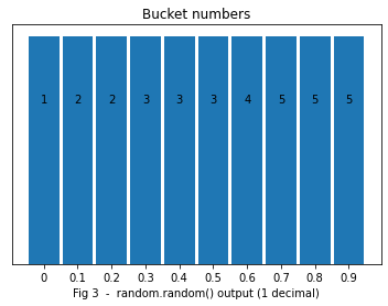
There is another way, with pros and cons. Instead of using buckets of varying widths, we could use identical buckets of width 0.1, and attribute x buckets to a number with a probability 0.x, as shown below in Fig 3.

Now, we can use the random number, rounded to 1 decimal, and use it to directly know which bucket (number) it corresponds. That can be done in O(1) using a dictionary.

For this example, the dictionary would be [0:1, 0.1:2 ,0.2:2 ,0.3:3 ,0.4:3 ,0.5:3 ,0.6:4 ,0.7:5 ,0.8:5 ,0.9:5]. We can think of the dictionary as a function that transforms the original pdf (probability density function) into a uniform one that can be sampled more easily.

Note that one can attribute any bucket to any number, as long as we attribute the right amount. For instance, [0:2, 0.1:5 ,0.2:2 ,0.3:3 ,0.4:3 ,0.5:3 ,0.6:4 ,0.7:5 ,0.8:5 ,0.9:1] would work just as well.

It seems like we have magically converted O(log n) into O(1) if we leave aside the time needed to create the dictionary. However, the last point is the kicker. If we use probabilities with 2 decimals, we need to create 100 buckets, 1,000 with 3 decimals so the complexity is actually O(2^nb_decimals + k). Note that, since we need at least one bucket for each number, 2^nb_decimals > n.

That sounds horrible suddenly, BUT the dictionary is created only once. If k grows, this approach becomes viable since k is not a multiplying factor.

It may seem that 5 or 6 decimals are a no-go, but, in many cases, if we need 6 decimals, many probabilities will be much smaller than others. A remedy to that situation, would be to group all numbers with a low probability in one small bucket (width = sum of their probabilities), to use 3 decimals for instance, and re-sample that bucket when we fall into it.

In my opinion, in such a case, taking any number randomly would be just as efficient. Imagine a particle filters with thousands of particles for instance. Many have low probabilities and it doesn’t matter if we select one of those particles or another.

However, in such case, the sampling probabilities change at every iteration. This technique would then have a complexity of O(2^nb_decimals * k). It is greater than O(k * n), so, here, this technique is not interesting. It shines when the dictionary is created once.

Code

I have used probabilities * 10 to get the number of times we need to repeat a number.

def random_generator(nums, probs, k=100000):

    all_nums = []
    # let's first create [1,2,3,3,3,4,5,5,5]
    for n,p in zip(nums, probs):
        all_nums += [n]*int(p*10)
            
    rnd_smpl = dict(enumerate(all_nums))        # our sampling dictionary
    
    sampling = dict(zip(nums,[0]*len(nums)))    # {1:0, 2:0, etc}
    
    for _ in range(k):
        sample = rnd_smpl[int(random()*10)]
        sampling[sample] += 1

    print(sampling)

random_generator([1,2,3,4,5],[0.1,0.2,0.3,0.1,0.3])
# {1: 10018, 2: 20253, 3: 30001, 4: 9983, 5: 29745}

Bonus

I recently saw a very astute way to physically sample a Normal distribution.

The video below shows a Galton Board.

Its hexagonal structure naturally makes the beads end up in the middle because there are more paths leading to the centre. In fact, since a bead can only fall to the right or to the left, it mimics the way Pascal triangles are built. The Pascal coefficients correspond to a binomial distribution, which approaches the Normal distribution, when the number of samples are high.

It’s not perfect since some beads are lost on the sides of the triangle, but it would be if one prevented that from happening. More info in Wikipedia.

I hope you liked my first article.

The next one will be about how to use Numpy vectorization for convolutions in Deep Learning by broadcasting a 2D meshgrid into a 6D one, for all convolutions with the kernel at every position to be calculated in parallel. Headache guaranteed!